3D Models

I created the 3d models, texture maps and bump maps for the lander, crashed lander and parachutes from scratch in Blender. UV unwrapping (mapping texture vertices to lander vertices) of the lander model proved difficult owing to the curved shape of the lander, as well as the 3d entry hatches and nose cone, however Blender's 3d texture painting feature helped with this dramatically, since I could paint directly onto the surface of the lander and parachutes.

I believe the original lander model for the c++ project was based upon the cone shaped Apollo Lander design, and as such I based my own design upon this. The models are loaded asynchronously by the three.js GLTF loader, and I spent a considerable amount of time reducing the polygon count of the lander mesh, in order to speed up the program. The fire for the exhaust was created using a volumetric fire library [1], which interpolates a series of texture image to produce the fire in 3d. I modified the original texture to include the blue flames on the back of the lander, and scaled the fire appropriately for varying thrust amounts, which made the lander look much more realistic.

Autopilot

Ascent

The ascent autopilot uses a gravity turn to put the rocket into either an aerostationary orbit, or into an orbit with a pre-specified apoapse and periapse.

The autopilot works by pitching the rocket over at a specified height this.pitchoverHeight and a specified angle this.pitchoverAngle, and then holding a pitch equal to the angle between the velocity and the rocket position vector until gravity reduces the radial velocity to zero. This is known as maintaining a zero angle of attack. A tangential burn is then executed, which sends the lander into an orbit whose apoapse is the apoapse of the final orbit to be reached. This is followed by a final burn which put the lander into the correct orbit.

In order to account for errors during the burn times, the lander uses an orbit stabilization system once in orbit. This performs short burns at any apse reached, which corrects opposite apse to the right altitude.
Because a gravity turn relies on only a pitchover angle and a pitchover height, it is much simpler than an actively controlled autopilot, but in general more fuel efficient, as by the time the rocket has fully pitched over, it is travelling at close to orbital velocity.
The main downside of a gravity turn is the uncontrollability of the trajectory after pitchover. I attempted to mitigate this by allowing the rocket to burn to orbit as soon as the tangential velocity approached zero, no matter the height.

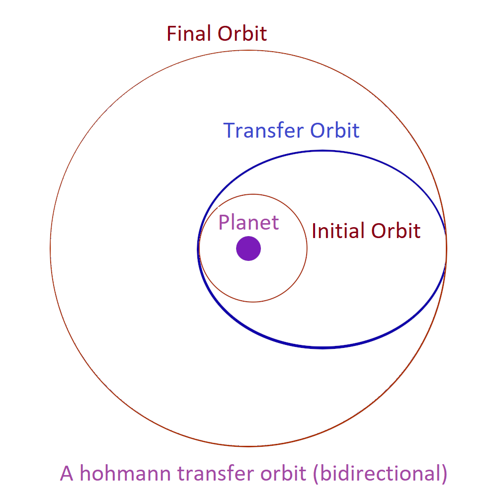
In order to calculate the burn length for each transfer, the autopilot performs each burn at an apse, and calculates the speed needed to put the lander into an elliptical Hohmann transfer orbit. This is the most fuel efficient method for a transfer between two orbits [6]. I decided to perform a fixed length burn rather than burning until the correct velocity is reached, as the inaccuracies of using a finite time burn combined with using the tangential velocity of the lander or using attitude stabilization to keep the lander perpendicular to its position vector sometimes had the unexpected consequence of making the lander spiral out of control, whereas a fixed length and direction burn had a much more predicable output.

Descent

The descent autopilot uses a PID controller programmed to aim towards a linear velocity decrease. I chose to use a PID autopilot due to its ability to cope with engine lag and delay, compared to a P autopilot. The lander is equipped with an altimeter which utilises the three.js raycaster to find the terrain height, and adjusts the autopilot accordingly.
There are four trainable parameters for the autopilot: kh , kp , ki and kd. These are respectively the height, proportional, integral and derivative gains.
Creating a working PID controller for the autopilot was one of the biggest challenges that I faced during the project. My main issue was with the integral part of the autopilot. When starting in a scenario, the zero starting velocity would add a negative buffer to the integral part, which would then cancel out the proportional and derivative controllers later, when the autopilot needed thrust.

This also worked in reverse. When the rocket slowed down after a long period of positive error (a speed too fast for the height) the integral controller would have a large positive offset, which would cause the rocket to continue thrusting, to the extent that it would start to rise again.
These errors caused problems during training the autopilot with the genetic algorithm too, as the smallest change in the integral controller could change an autopilot from stable to oscillating, or even heading back off into space.

I experimented with a staged autopilot, which would only allow the integral controller to start after the parachute had been deployed and the error was positive, however this proved cumbersome and difficult to make stable in all scenarios. Eventually I worked out that to allow the integral controller to slow the rocket down, but not excessively, I needed to compute a running sum of errors for the integral, and reset this to zero every time the current error was below zero. This was because a rocket is not a conventional PID controller set up - without an infinite range of thrust values available, it was possible for a pure integral controller to put the final error value so low or high that correct would be impossible.

For the thrust to balance the rocket with zero error, a value for the thrust offset DELTA needed to be computed. This was originally equal to the max weight of the rocket divided by the max thrust, however this presented difficulties when using large amounts of fuel on descent, as the rocket would become much lighter. I therefore modified the offset value constantly to reflect the new weight of the rocket, which balanced the weight of the rocket more effectively, no matter the height.

Genetic Algorithm

In order to train the autopilot, I wrote a genetic algorithm from scratch, first in c++ in the original project, then in JavaScript ( to be run in node.js offline).

The stages of this genetic algorithm are as follows:

• First a population of autopilots objects is created: new COEFFS( Math.random(), Math.random(), Math.random(), Math.random())
• Then each autopilot is tested and is assigned a fitness attribute, based on the performance factor which is being trained. In this algorithm, any pilot reaching a descent velocity of 0 before landing was given a fitness of zero, as well as any crashed autopilots.
• During this, the total fitnesses from each autopilot are summed, to give a totalPopFitness. The algorithm then iterates through the list of autopilots and assigns each one a cumulative fitness fraction sumFitness/totalPopFitness. Those autopilots with a higher fitness will have a larger amount of numbers which are closer to themselves than any other autopilot. This means that they are more likely to be the closest number to a random number picked, and so are more likely to be selected. This method also has the benefit that raw fitness values do not have to be in any particular range, as long as higher fitnesses are better autopilots.
• To create each autopilot in the next (improved) generation, two random numbers are selected, and the algorithm finds the autopilot with a cumulative fitness fraction closest to the selected number. These are the parents for the next generation.
• The two parents then swap half of their coefficients, forming two child autopilots. There is also a chance of mutation, which I generally set around 10-30% . A mutation coefficient multiplies the coefficient value by a factor in the interval [0.8-1.2], in order to ensure that coefficients stay roughly of the same magnitude, and do not completely unbalance the others. In general the autopilot coefficients stay within the interval (0,10), although on occasion some briefly went higher.
• Instead of creating the entire next generation from this process, the best and second best autopilots from the last generation are included unchanged into the next generation. This is known as elitism, and helps the genetic algorithm avoid stagnation upon coming close to the peak fitness possible.

One of the problems I encountered was the propagation of "fluky" autopilots. Essentially, an autopilot with badly trained coefficients would landed due to random wind effects, and the elitism in the genetic algorithm would carry the autopilot into the next generation, when it was in fact unstable. To counter this I decided to test each autopilot with a random terrain height (2e5 - 1e4) *Math. random() + 1e4 a number of times, (up to 6), and multiply the resultant fitness values together.

I also started each autopilot at slightly varying heights, between 10000m and 200000m, in order to ensure that each autopilot could cope with landings from an height, and was not overly adapted to a specific scenario. This ensured that any autopilot with a fitness value above zero was consistently able to survive random terrain and wind, as had it failed even one out of six tests, its fitness was reduced to zero. The algorithm was able to train all four autopilot parameters, kh , kp , ki and kd.

I set the fitness of an autopilot to zero if the velocity ever reached zero before landing. This was because any autopilot that paused in mid air would be automatically worse than one with a smooth descent. Additionally, this change was caused by my initial difficulties with the integral autopilot, as the integral controller had a tendency originally to send the lander back off into orbit. The condition still proved somewhat effective at removing oscillating autopilots, where the D or I values were too high, which made the autopilots constantly overshoot their target velocities. When training the autopilots, the value of dt used in the simulation greatly affected some of the results. This was because whilst the online versions run on a dt of 0.001, the offline versions originally ran on a dt of 1, which resulted in inaccurate autopilots. Changing dt to 0.001 proved much too slow in training, but 0.01 was a suitable compromise.

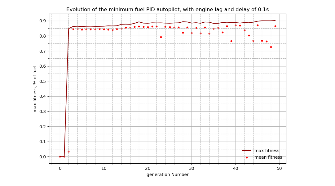
The graph below shows 25 autopilots being trained for 50 generations. The jump at generation 3 occurs as the algorithm finds its first autopilot that works, essentially getting lucky with such a high fitness. The algorithm improves gradually, with a series of plateaus, which represent regions where no mutations were present, and reaches a maximum around the 90% mark for fuel usage.

Although the algorithm appears to still be improving towards generation 50, it can be seen from the diverging mean fitness values that the autopilot has in fact reached close to its peak performance, because this algorithm implements elitism, which passes through the best autopilots from each generation to the next without any changes. This means that while the best autopilots should always improve slowly, the mean performance will fall when the maximum fitness possible is approached, as any changes to the best autopilots will reduce the fitness instead of improving it, resulting in a lower mean fitness.

Performance vs hand tuning

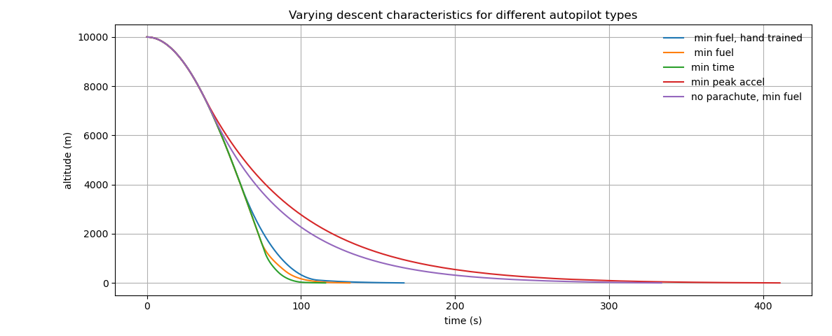
Having laboriously hand trained the PID autopilots initially, I was astonished at first at the improvements the genetic algorithm made over hand tuning. The following graph shows the effect of training the autopilot on its descent characteristic. The graphs follow an unnervingly neat pattern, with the minimum time autopilot landing first, followed by the minimum fuel autopilot, and my hand trained P only controller.
Interestingly, the minimum time and minimum fuel autopilots were particularly close together, since in reality, the optimum burn pattern for a rocket landing is the "suicide burn" approach, in which the throttle is applied at maximum from the last possible opportunity until landing, resulting in the fastest and most fuel efficient method of landing.
It can also be seen from these graphs that the minimum time autopilot comes close to being the most efficient autopilot possible. This can be seen from the point at which the graph diverges from the descent curve - this height is so close to ground level with the time autopilot that were it to be any lower, it is doubtful whether the lander could slow down in time to land even at max thrust, much less avoid the changing terrain.

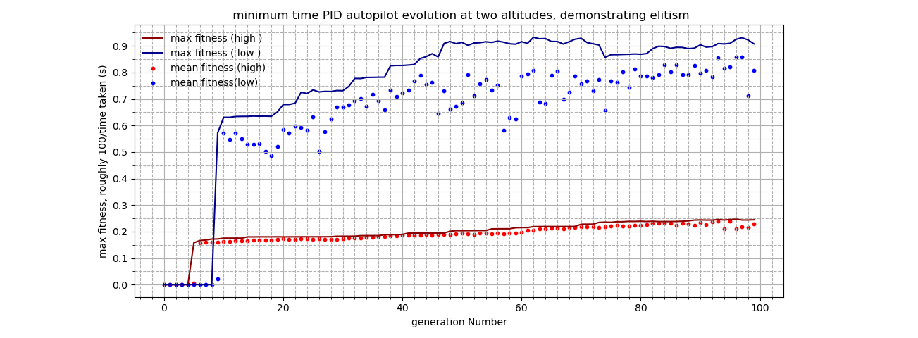
The problem of changing terrain on the autopilots is highlighted well by the following graph, which shows the training of two minimum time autopilots, from different starting altitudes: a low of 10000m and a high of 200000m. The effect this has on the fitness of the resulting autopilots is clear - for the low start autopilot (blue), the mean values for the autopilots have a much wider deviation from the max fitness line. This is because the low start autopilot, when training, has a high tendency to crash on unfamiliar terrain due to its optimisation for low and late thrust, compared to the high start autopilot, for which the changing terrain comprises a much smaller proportion of the descent.

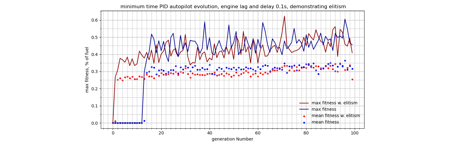
The effects of elitism

I was interested to learn the effects of elitism on the genetic algorithm, in order to speed up the training process, and force permanent autopilot growth without a falloff in later generations. Whilst the obvious effect of forcing near constant improvement due to the duplication of the last generations autopilots is clearly shown in the graphs above - the effect of the elitism on performance is better shown by the two graphs below.

The first graph shows a minimum time autopilot being trained with and without elitism. The starting heights are all random, hence the spikiness of the graphs, however a few trends are visible. The mean scores for the autopilot without elitism are almost flat. They show next to no increase as the generations progress, however the mean elitist fitnesses increase much more steadily. This is most likely due to the saturation of the elitist algorithm with improved autopilots as the generations progress.
The elitist algorithm also shows a greater tendency towards improvement here, and despite starting worse, begins to outperform the non-elitist algorithm in later generations.

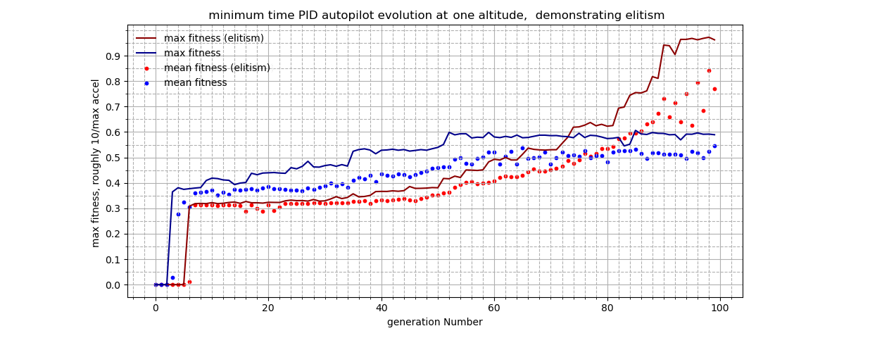
The second graph shows the effect of elitism on the training of a single minimum time autopilot, but this time at one single height. Dips and troughs can be seen in the non-elitist graph, and the algorithm fails to converge to the maximum possible fitness. On the other hand, the elitist graph shows almost no marked dips, except very near its peak, and converges to the maximum value. Whilst there is always a possibility of this being through luck, the probability of the elitist algorithm finding the fittest autopilots is considerably increased as the best autopilots are always preserved intact, and therefore have a higher "lifetime" within the algorithm, meaning they make a greater impact on successive generations, and serve as building blocks for their mutations, unlike a non-elitist algorithm, which only has similar if not mutated children in each generation.

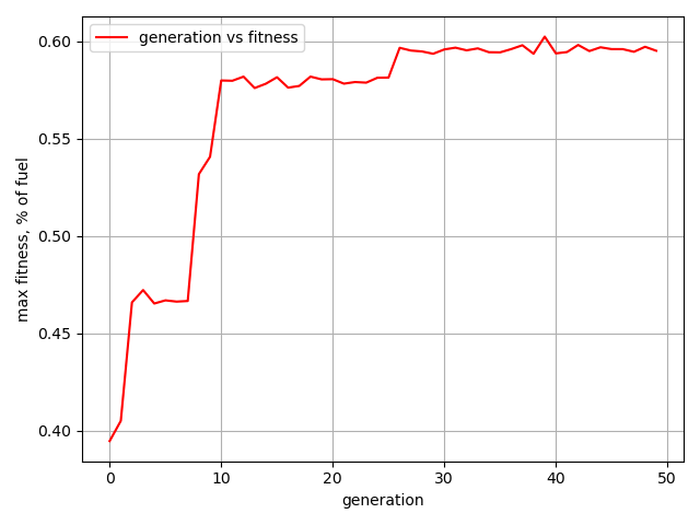
This final training graph shows one of the earlier autopilot training sessions, with a very low but violent mutation rate and elitism, but a relatively small pool of only 25 per generation. The effect that the sporadic mutations have on the lander is evident - the improvements come in chunks, with flat plateaus, rather than a smooth or jumpy increase.
This sort of behaviour is bad for a genetic algorithm as the algorithm cannot converge, instead jumping between values, and also does not create enough genetic diversity within each population to improve beyond a certain point, as the algorithm becomes saturated with copies of the same autopilot.

Fitness values

One of the main benefits to a genetic algorithm, was the ability to easily specify a custom fitness function for each training generation. I specified the initial fitness functions as follows:

Since one of my problems whilst training the algorithm was its inability to produce consistent autopilots, instead of landings based on pure luck, I modified the algorithm to test each autopilot multiple times from different heights and on different terrains.

Given an autopilot to test, the fitness for the first trial is calculated. It is then multiplied by the fitness from the next test, and so on until a total fitness is reached. This means an autopilot must pass all tests before achieving a fitness score above zero.

Planet Texture

Thanks to the Planetary Pixel Emporium [2] for the planet textures. The Martian surface used a chunk handler method to extend a flat plane of terrain in the direction of the lander's flight across the surface. The chunks were created in a web worker, and the coordinates loaded asynchronously back into the world.
This can occasionally result in the lander "landing" on a surface minus the terrain, however this is mostly down to the speed of terrain rendering on an individual computer.

Once loaded from the web worker, the chunks are tiled together on a flat plane underneath the lander representing the planet's surface. This approach did lead to working terrain generation, however if the lander travels too far over the surface, its altitude increases, as in the world space it is not travelling around the Mars surface, but in a straight line tangential to it. This is however barely noticeable in the simulation, and it would in theory be possible to tile the terrain around the planet surface.

The surface itself uses 3 layers of simplex noise, in order to create a terrain which was rough locally but smooth globally. I coloured each individual vertex separately, in order to achieve a smooth colour across the surface, despite there being a minimal polygon count for each terrain chunk. I added a randomness to the colour of each vertex based off its absolute position, so that although each vertex has a random element to its colour, along chunk boundaries the colours are aligned, and so the boundary is hidden.

Overall, using a web worker allowed the computationally complex work of generating terrain coordinates to be done asynchronously, which sped up the simulation greatly. I had also thought to run the physics engine in a web worker, however this would take too much time between calls and responses to be a great improvement.
On the other hand, a much more useful future implementation could be using a web worker to run the genetic algorithm online, thus allowing users to train the autopilots themselves, and adjust parameters as wished. Although I did not have time to add this feature, I do not believe it would be that difficult, as a simple call and response at the start and end of a training session would suffice to connect the main file and the web worker.

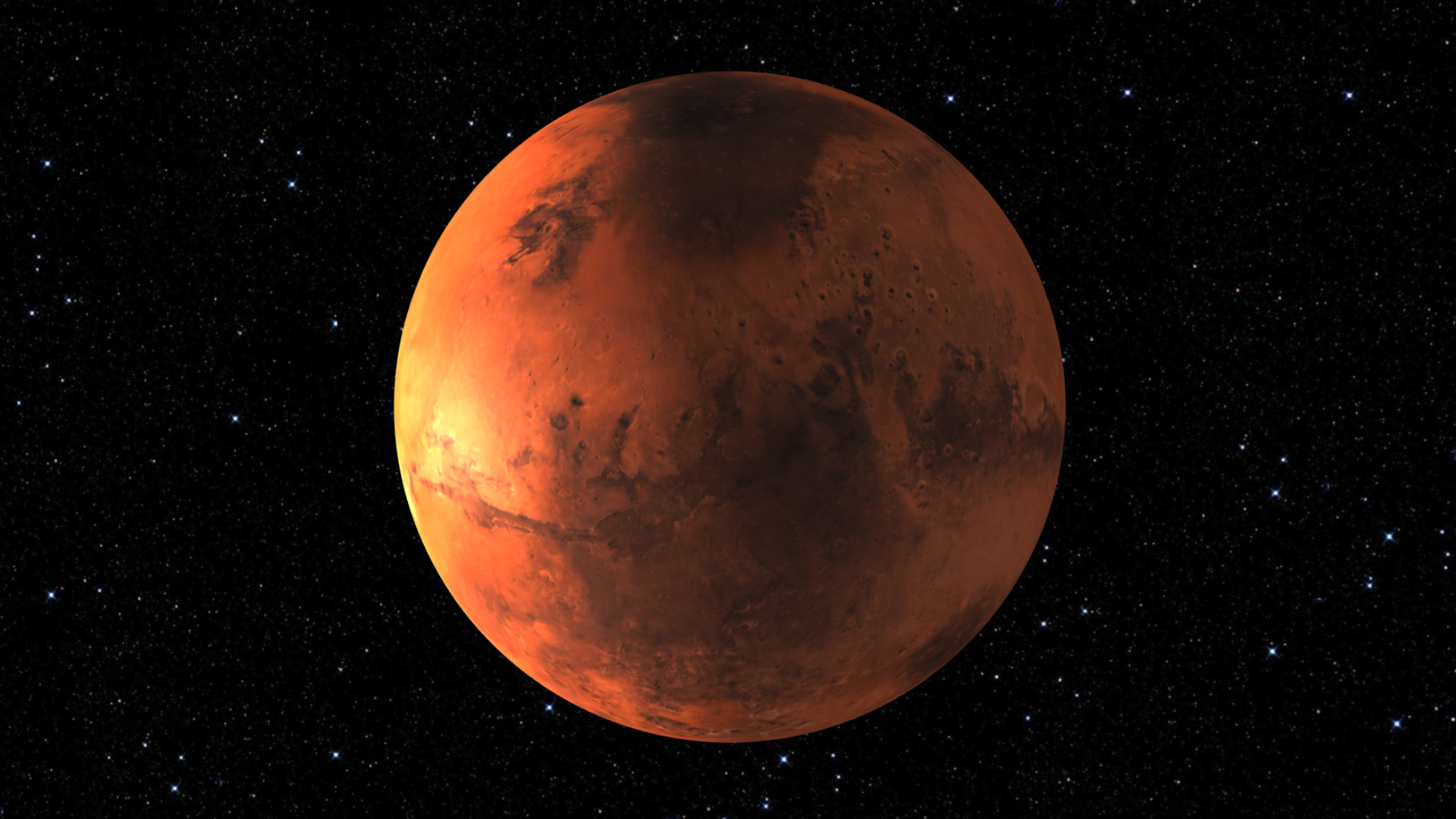
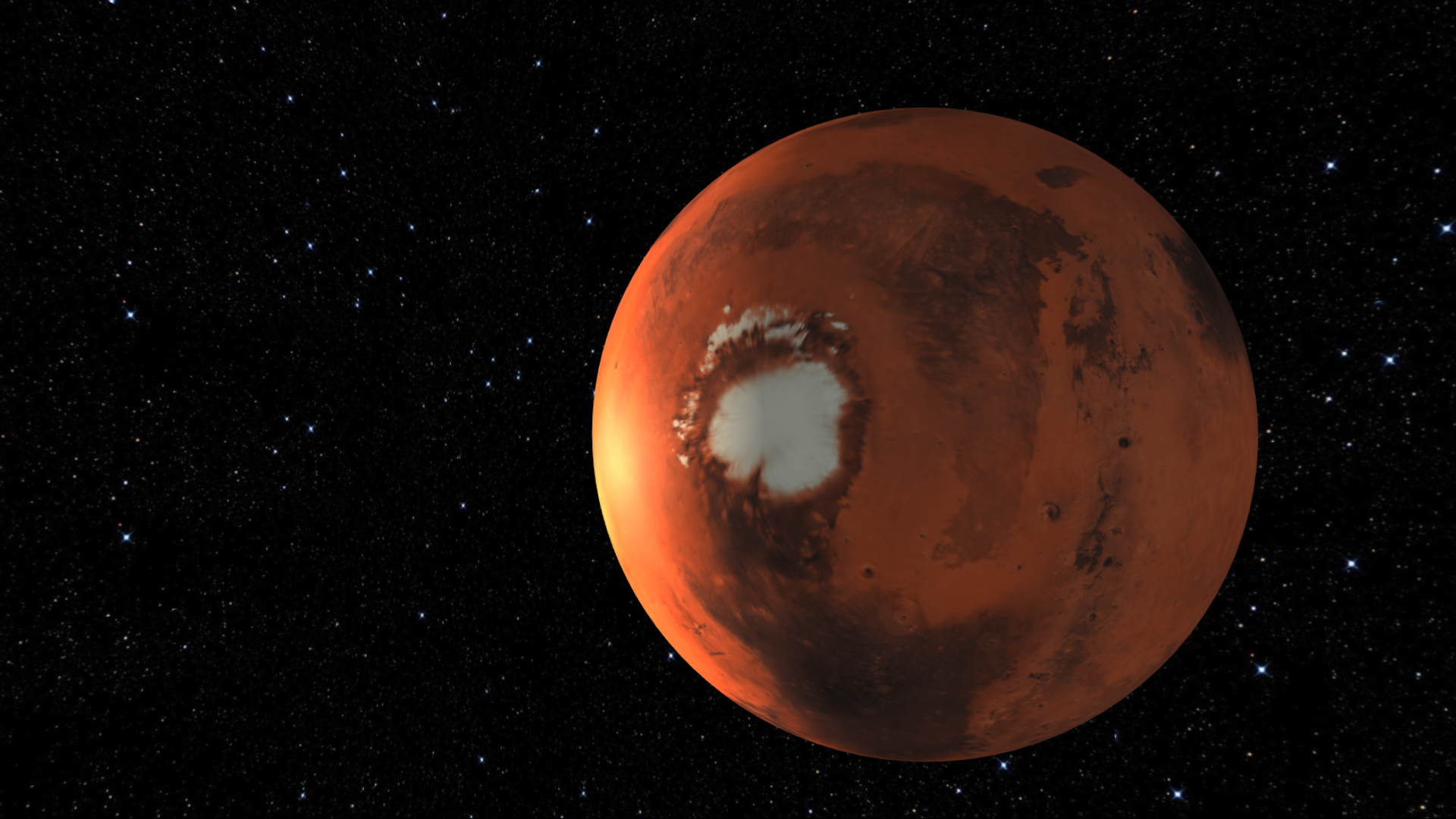
The below image shows the Martian poles, which due to the spherical texture mapping and the fact that the planet is not perfectly symmetrical, have some distortions. Despite this, I think that the planets work well, especially considering that they are rendered in three.js to a 1:1 scale.

Wind

Whilst investigating suitable wind models to use for the planet, I came across the Mars Climate Database [3]. Whilst I eventually only took guidelines from this as to the magnitude of the Martian winds, the information proved extremely useful, and I would encourage anyone else attempting a project along these lines to take a look. Eventually I decided on a GCM ( global climate model ) for the main planetary winds. The main wind patterns can be seen here [4], and I added a random scale on top of this, as well as random gust generation. The main principle of the GCM I used was that of Hadley Cell Circulation, between the poles and the equator. The stages to my implementation were:

• First the direction of the wind flow from the pole to the equator is calculated
• Then the wind vector is scaled, depending on its height above the Martian surface, following a cubic formula, shown below. 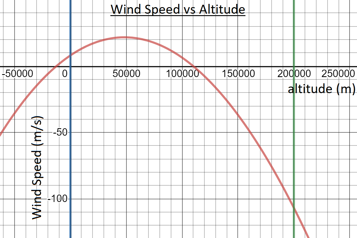This represents the way in which winds circulate back over themselves high in the atmosphere.
• Then a random wind variation vector is created. This is scaled so that acts *almost* in the plane, but creates a slight updraft or downdraft.
• The two vectors are then added together to form the total normal wind speed.
• Similar to the wind variation vector, a gust direction vector is also created, and scaled to act *almost* in the plane. This is then multiplied by a separate gustScale. With a simplex noise function gustScale = noise. simplex2 ( time / timeScale , 0) , the gusts can be timed to occur only at positive values of gustScale. This also ensures that by using gustScale, the magnitude of the gust vector, the gusts fade in and out.
• The wind and gust vectors are then added together to get the final wind speed. Winds do not occur outside the exosphere, since there is no atmosphere there, and due to the lack of atmospheric rotation, I did not include a Coriolis wind velocity.

The randomness in the wind is created by a simplex noise implementation in JavaScript [5]. Gusts fade in and out, and are timed randomly, by only appearing at positive values of another noise function.

Rotation

The Rotation of the lander was possibly one of the hardest problems to overcome, as this was the first time that I had encountered quaternions, and 3D rotation in general. I originally tried to rotate the lander about axis that were fixed with the lander group, but this proved disastrously unintuitive, and untrue to real life, as thrusters would be fixed on the rocket body. Eventually I worked out how to rotate the lander around its own axis, by first generating an angular momentum for the world in the world coordinates, then transforming this to a rotation in the lander coordinates. Unfortunately, the rotation of the lander does not affect its dynamics beyond vectoring the thrust, however this is something that could definitely be added, albeit at a considerable increase in complexity.

Other Notable Points

• I managed to include custom scenario creation in this version of my Mars lander project, however this can be a somewhat temperamental feature at times, when combined with the ascent autopilot. I had to decide between adding more functionality, and adding less usability, as I could easily have added the option for orientation control, or even customisable engine lag and delay. I finally decided that these features were more time than use, leaving them out in the final version.
• The directional lighting is a commonly used technique for simulating the sun, which creates some lovely effects as the planet turns. I found out whilst making performance improvements to the code, that in order to add and remove lights from the scene it is better to write: light.visible = false than: scene.remove(light); as manipulating the scene has a much higher performance overhead compared to changing individual properties.
• Instead of opting for THREE.OrbitControls with a fixed "up" axis, I decided to use the slightly less intuitive but more flexible THREE.TrackballControls. These make it slightly harder to orient the lander in the window, but have the benefit of providing more camera angles from which to view the scene. I finally settled with trackball controls for orbit, and a more intuitive orbit control setup for landing, which also meant that users cannot easily view beneath the terrain, which would spoil the realism of the game.
• Instead of using a scaled down planet as I the c++ version, I used three.js' support for logarithmic depth buffering. This enabled me to scale Mars and the lander at a 1:1 scale.
• Due to the way in which three.js fog gets denser further from the camera, when transitioning to the planet surface, I changed the opacity of the sky and planet to give the appearance of fog, before switching to three.js fog for the planet surface.
• The world view is a new THREE.Scene() and renderer, that is called in the main loop. The past positions are coloured according to their distance along the line, and the user has the option to switch between planet and lander focus mode. The wind arrow is also a new THREE.Scene() and renderer, which uses the same camera orientation and position (scaled down) as the lander, in order to rotate with it.

Future Improvements

The Parachute

When training my algorithm, I initially sought to automate the deployment of the parachute by simply deploying it as soon as was safe to do so, to reduce the fuel needed for landing. When training the autopilots, I achieved very satisfactory results by allowing the parachute to be deployed as soon as the error was positive, and the speed was safe to do so - and if not, then throttling 100% until this was possible. This worked because by adjusting kh, the genetic algorithm was able in effect to alter the height at which the parachute was deployed.

The downside to this is that the parachute deployment altitude is not a trainable parameter, and as such could have removed some of the flexibility that the genetic algorithm might have found when training the autopilots separately, especially in the case of minimum time autopilots.

The Ascent Autopilot

Whilst using a gravity turn for an ascent autopilot does achieve one of the most fuel efficient launches, it is by no means the absolute best way to launch, and can easily be affected by factors such as wind and atmospheric rotation (which is absent in this simulation). The ascent autopilot which I originally tried to implement in the c++ versions used a similar PID controller to copy the gravity turn trajectory, but this proved extremely difficult to implement, as the gravity turn equations cannot be integrated except numerically, and without a trajectory to lock onto, the PID controller could not control both the thrust and pitch angle of the rocket.

On that note, I did not manage to add atmospheric rotation into this project, despite it being present in the c++ version. This was due to the way in which I generated the terrain, which would not be able to a) generate fast enough or b) generate spherically around the Mars radius, had I added rotation. Given more time however, I would have been interested to try and generate the terrain spherically to allow rotation, since the only modifications would be the location of the terrain chunks, and the method of generating the vertices. Additionally, my GCM does not account for the Coriolis atmospheric rotation which would be present in a real life atmosphere, as this cannot be done without fully implementing atmospheric rotation.

The last thing which would have been a nice small touch to implement would have been a more gradual increase to the wind velocity when entering the exosphere. The current GCM starts the wind immediately the lander enters the exosphere, which is naturally unrealistic.

Overall, I found this project to be a brilliant learning experience for programming, front end web development and graphics. Since this was my first time using three.js, OpenGL, c++ and the trio of HTML, CSS and JavaScript, I am massively pleased that the overall project went so smoothly in hindsight, and hope to continue projects like this in the future!